Random variable is a variable that can take on certain values depending on various circumstances, and random variable is called continuous , if it can take any value from some bounded or unbounded interval. For a continuous random variable, it is impossible to specify all possible values, therefore, the intervals of these values that are associated with certain probabilities are denoted.
Examples of continuous random variables are: the diameter of a part turned to a given size, the height of a person, the range of a projectile, etc.
Since for continuous random variables the function F(x), Unlike discrete random variables, has no jumps anywhere, then the probability of any single value of a continuous random variable is equal to zero.
This means that for a continuous random variable it makes no sense to talk about the probability distribution between its values: each of them has zero probability. However, in a certain sense, among the values of a continuous random variable there are "more and less probable". For example, it is unlikely that anyone will doubt that the value of a random variable - the height of a randomly encountered person - 170 cm - is more likely than 220 cm, although one and the other value can occur in practice.
Distribution function of a continuous random variable and probability density
As a distribution law, which makes sense only for continuous random variables, the concept of distribution density or probability density is introduced. Let's approach it by comparing the meaning of the distribution function for a continuous random variable and for a discrete random variable.
So, the distribution function of a random variable (both discrete and continuous) or integral function is called a function that determines the probability that the value of a random variable X less than or equal to limit value X.
For a discrete random variable at the points of its values x1 , x 2 , ..., x i ,... concentrated masses of probabilities p1 , p 2 , ..., p i ,..., and the sum of all masses is equal to 1. Let's transfer this interpretation to the case of a continuous random variable. Imagine that a mass equal to 1 is not concentrated at separate points, but is continuously "smeared" along the x-axis Ox with some uneven density. The probability of hitting a random variable on any site Δ x will be interpreted as the mass attributable to this section, and the average density in this section - as the ratio of mass to length. We have just introduced an important concept in probability theory: the distribution density.
Probability Density f(x) of a continuous random variable is the derivative of its distribution function:
![]() .
.
Knowing the density function, we can find the probability that the value of a continuous random variable belongs to the closed interval [ a; b]:

the probability that a continuous random variable X will take any value from the interval [ a; b], is equal to a certain integral of its probability density in the range from a before b:
![]()
![]() .
.
In this case, the general formula of the function F(x) the probability distribution of a continuous random variable, which can be used if the density function is known f(x) :
![]() .
.
The graph of the probability density of a continuous random variable is called its distribution curve (fig. below).

The area of the figure (shaded in the figure), bounded by a curve, straight lines drawn from points a and b perpendicular to the abscissa axis, and the axis Oh, graphically displays the probability that the value of a continuous random variable X is within the range of a before b.
Properties of the probability density function of a continuous random variable
1. The probability that a random variable will take any value from the interval (and the area of \u200b\u200bthe figure, which is limited by the graph of the function f(x) and axis Oh) is equal to one:
2. The probability density function cannot take negative values:
and outside the existence of the distribution, its value is zero
Distribution density f(x), as well as the distribution function F(x), is one of the forms of the distribution law, but unlike the distribution function, it is not universal: the distribution density exists only for continuous random variables.
Let us mention the two most important in practice types of distribution of a continuous random variable.
If the distribution density function f(x) a continuous random variable in some finite interval [ a; b] takes a constant value C, and outside the interval takes on a value equal to zero, then this distribution is called uniform .
If the graph of the distribution density function is symmetrical about the center, the average values are concentrated near the center, and when moving away from the center, more different from the averages are collected (the graph of the function resembles a cut of a bell), then this distribution is called normal .
Example 1 The probability distribution function of a continuous random variable is known:
Find a feature f(x) the probability density of a continuous random variable. Plot graphs for both functions. Find the probability that a continuous random variable will take any value in the range from 4 to 8: .
Solution. We obtain the probability density function by finding the derivative of the probability distribution function:

Function Graph F(x) - parabola:

Function Graph f(x) - straight line:

Let's find the probability that a continuous random variable will take any value in the range from 4 to 8:
Example 2 The probability density function of a continuous random variable is given as:

Calculate factor C. Find a feature F(x) the probability distribution of a continuous random variable. Plot graphs for both functions. Find the probability that a continuous random variable will take any value in the range from 0 to 5: .
Solution. Coefficient C we find, using property 1 of the probability density function:
Thus, the probability density function of a continuous random variable is:
Integrating, we find the function F(x) probability distributions. If a x < 0 , то F(x) = 0 . If 0< x < 10 , то
![]() .
.
x> 10 , then F(x) = 1 .
Thus, the full record of the probability distribution function is:
Function Graph f(x) :

Function Graph F(x) :

Let's find the probability that a continuous random variable will take any value in the range from 0 to 5:
Example 3 Probability density of a continuous random variable X is given by equality , while . Find coefficient BUT, the probability that a continuous random variable X takes some value from the interval ]0, 5[, the distribution function of a continuous random variable X.
Solution. By condition, we arrive at the equality

Therefore, whence . So,
![]() .
.
Now we find the probability that a continuous random variable X will take any value from the interval ]0, 5[:
Now we get the distribution function of this random variable:

Example 4 Find the probability density of a continuous random variable X, which takes only non-negative values, and its distribution function ![]() .
.
Concepts of mathematical expectation M(X) and dispersion D(X) introduced earlier for a discrete random variable can be extended to continuous random variables.
· Mathematical expectation M(X) continuous random variable X is defined by the equality:
provided that this integral converges.
· Dispersion D(X) continuous random variable X is defined by the equality:
· Standard deviationσ( X) continuous random variable is defined by the equality:
All the properties of mathematical expectation and dispersion considered earlier for discrete random variables are also valid for continuous ones.
Problem 5.3. Random value X given by the differential function f(x):
Find M(X), D(X), σ( X), as well as P(1 < X< 5).
Solution:
M(X)= =
+ = 8/9 0+9/6 4/6=31/18,
D(X)=
= = /
P 1 =
Tasks
5.1. X
f(x), as well as
R(‒1/2 < X< 1/2).
5.2. Continuous random variable X given by the distribution function:
Find the differential distribution function f(x), as well as
R(2π /9< X< π /2).
5.3. Continuous random variable X
Find: a) number With; b) M(X), D(X).
5.4. Continuous random variable X given by the distribution density:
Find: a) number With; b) M(X), D(X).
5.5. X:
Find: a) F(X) and plot its graph; b) M(X), D(X), σ( X); c) the probability that in four independent trials the value X takes exactly 2 times the value belonging to the interval (1;4).
5.6. Given the probability distribution density of a continuous random variable X:
Find: a) F(X) and plot its graph; b) M(X), D(X), σ( X); c) the probability that in three independent trials the value X will take exactly 2 times the value belonging to the interval .
5.7. Function f(X) is given as:
With X; b) distribution function F(x).
5.8. Function f(x) is given as:
Find: a) the value of the constant With, at which the function will be the probability density of some random variable X; b) distribution function F(x).
5.9. Random value X, concentrated on the interval (3;7), is given by the distribution function F(X)= X takes the value: a) less than 5, b) not less than 7.
5.10. Random value X, concentrated on the interval (-1; 4), is given by the distribution function F(X)= . Find the probability that the random variable X takes the value: a) less than 2, b) less than 4.
5.11.
Find: a) number With; b) M(X); c) probability R(X > M(X)).
5.12. The random variable is given by the differential distribution function:
Find: a) M(X); b) probability R(X ≤ M(X)).
5.13. The Time distribution is given by the probability density:
Prove that f(x) is indeed a probability density distribution.
5.14. Given the probability distribution density of a continuous random variable X:
Find a number With.
5.15. Random value X distributed according to Simpson's law (isosceles triangle) on the segment [-2; 2] (Fig. 5.4). Find an analytical expression for the probability density f(x) on the whole number line.
Rice. 5.4 Fig. 5.5
5.16. Random value X distributed according to the "right triangle" law in the interval (0; 4) (Fig. 5.5). Find an analytical expression for the probability density f(x) on the whole number line.
Answers
P (-1/2<X<1/2)=2/3.
P(2π /9<X< π /2)=1/2.
5.3. a) With=1/6, b) M(X)=3 , c) D(X)=26/81.
5.4. a) With=3/2, b) M(X)=3/5, c) D(X)=12/175.
b) M(X)= 3 , D(X)= 2/9, σ( X)= /3.
b) M(X)=2 , D(X)= 3 , σ( X)= 1,893.
5.7. a) c = ; b)
5.8. a) With=1/2; b)
5.9. a) 1/4; b) 0.
5.10. a) 3/5; b) 1.
5.11. a) With= 2; b) M(X)= 2; in 1- ln 2 2 ≈ 0,5185.
5.12. a) M(X)= π /2 ; b) 1/2
Chapter 1. Discrete random variable
§ 1. The concept of a random variable.
The law of distribution of a discrete random variable.
Definition : Random is a quantity that, as a result of the test, takes only one value out of a possible set of its values, unknown in advance and depending on random causes.
There are two types of random variables: discrete and continuous.
Definition : The random variable X is called discrete (discontinuous) if the set of its values is finite or infinite, but countable.
In other words, the possible values of a discrete random variable can be renumbered.
You can describe a random variable using its distribution law.
Definition : The distribution law of a discrete random variable called the correspondence between the possible values of a random variable and their probabilities.
The distribution law of a discrete random variable X can be given in the form of a table, in the first line of which all possible values of the random variable are indicated in ascending order, and in the second line the corresponding probabilities of these values, i.e.
where р1+ р2+…+ рn=1
Such a table is called a series of distribution of a discrete random variable.
If the set of possible values of a random variable is infinite, then the series р1+ р2+…+ рn+… converges and its sum is equal to 1.
The distribution law of a discrete random variable X can be depicted graphically, for which a polygonal line is built in a rectangular coordinate system, connecting successively points with coordinates (xi;pi), i=1,2,…n. The resulting line is called distribution polygon (Fig. 1).
Organic chemistry "href="/text/category/organicheskaya_hiimya/" rel="bookmark"> of organic chemistry are 0.7 and 0.8, respectively. Draw up the law of distribution of the random variable X - the number of exams that the student will pass.
Solution. As a result of the exam, the considered random variable X can take one of the following values: x1=0, x2=1, x3=2.
Let's find the probability of these values. Denote the events:
https://pandia.ru/text/78/455/images/image004_81.jpg" width="259" height="66 src=">
 |
So, the distribution law of the random variable X is given by the table:
Control: 0.6+0.38+0.56=1.
§ 2. Distribution function
A complete description of a random variable is also given by the distribution function.
Definition: The distribution function of a discrete random variable X the function F(x) is called, which determines for each value x the probability that the random variable X takes a value less than x:
F(x)=P(X<х)
Geometrically, the distribution function is interpreted as the probability that the random variable X will take the value that is depicted on the number line by a point to the left of the point x.
1)0≤F(x)≤1;
2) F(x) is a non-decreasing function on (-∞;+∞);
3) F(x) - continuous from the left at the points x= xi (i=1,2,…n) and continuous at all other points;
4) F(-∞)=P (X<-∞)=0 как вероятность невозможного события Х<-∞,
F(+∞)=P(X<+∞)=1 как вероятность достоверного события Х<-∞.
If the distribution law of a discrete random variable X is given in the form of a table:
then the distribution function F(x) is determined by the formula:
https://pandia.ru/text/78/455/images/image007_76.gif" height="110">
0 for x≤ x1,
p1 at x1< х≤ x2,
F(x)= p1 + p2 at x2< х≤ х3
1 for x> xn.
Its graph is shown in Fig. 2:

§ 3. Numerical characteristics of a discrete random variable.
Mathematical expectation is one of the important numerical characteristics.
Definition: Mathematical expectation M(X) Discrete random variable X is the sum of the products of all its values and their corresponding probabilities:
M(X) = ∑ xiрi= x1р1 + x2р2+…+ xnрn
Mathematical expectation serves as a characteristic of the average value of a random variable.
Properties of mathematical expectation:
1)M(C)=C, where C is a constant value;
2) M (C X) \u003d C M (X),
3)M(X±Y)=M(X)±M(Y);
4)M(X Y)=M(X) M(Y), where X, Y are independent random variables;
5)M(X±C)=M(X)±C, where C is a constant value;
To characterize the degree of dispersion of possible values of a discrete random variable around its mean value, variance is used.
Definition: dispersion D ( X ) random variable X is the mathematical expectation of the squared deviation of the random variable from its mathematical expectation:
Dispersion properties:
1)D(C)=0, where C is a constant value;
2)D(X)>0, where X is a random variable;
3)D(C X)=C2 D(X), where C is a constant value;
4)D(X+Y)=D(X)+D(Y), where X, Y are independent random variables;
To calculate the variance, it is often convenient to use the formula:
D(X)=M(X2)-(M(X))2,
where М(Х)=∑ xi2рi= x12р1 + x22р2+…+ xn2рn
The variance D(X) has the dimension of the square of a random variable, which is not always convenient. Therefore, the value √D(X) is also used as an indicator of the dispersion of possible values of a random variable.
Definition: Standard deviation σ(X) random variable X is called the square root of the variance:
![]()
Task number 2. The discrete random variable X is given by the distribution law:
Find P2, the distribution function F(x) and plot its graph, as well as M(X), D(X), σ(X).
Solution: Since the sum of the probabilities of the possible values of the random variable X is equal to 1, then
Р2=1- (0.1+0.3+0.2+0.3)=0.1
Find the distribution function F(x)=P(X Geometrically, this equality can be interpreted as follows: F(x) is the probability that a random variable will take the value that is depicted on the real axis by a point to the left of x. If x≤-1, then F(x)=0, since there is not a single value of this random variable on (-∞;x); If -1<х≤0, то F(х)=Р(Х=-1)=0,1, т. к. в промежуток (-∞;х) попадает только одно значение x1=-1; If 0<х≤1, то F(х)=Р(Х=-1)+ Р(Х=0)=0,1+0,1=0,2, т. к. в промежуток (-∞;х) two values x1=-1 and x2=0 fall; If 1<х≤2, то F(х)=Р(Х=-1) + Р(Х=0)+ Р(Х=1)= 0,1+0,1+0,3=0,5, т. к. в промежуток (-∞;х) попадают три значения x1=-1, x2=0 и x3=1; If 2<х≤3, то F(х)=Р(Х=-1) + Р(Х=0)+ Р(Х=1)+ Р(Х=2)= 0,1+0,1+0,3+0,2=0,7, т. к. в промежуток (-∞;х) попадают четыре значения x1=-1, x2=0,x3=1 и х4=2; If x>3, then F(x)=P(X=-1) + P(X=0)+ P(X=1)+ P(X=2)+P(X=3)= 0.1 +0.1+0.3+0.2+0.3=1, since four values x1=-1, x2=0,x3=1,x4=2 fall into the interval (-∞;x) and x5=3. https://pandia.ru/text/78/455/images/image006_89.gif" width="14 height=2" height="2"> 0 for x≤-1, 0.1 at -1<х≤0, 0.2 at 0<х≤1, F(x)= 0.5 at 1<х≤2, 0.7 at 2<х≤3, 1 for x>3 Let's represent the function F(x) graphically (Fig. 3): https://pandia.ru/text/78/455/images/image014_24.jpg" width="158 height=29" height="29">≈1.2845. §
4. Binomial distribution law discrete random variable, Poisson's law. Definition: Binomial
called the law of distribution of a discrete random variable X - the number of occurrences of event A in n independent repeated trials, in each of which event A may occur with probability p or not occur with probability q = 1-p. Then Р(Х=m)-probability of occurrence of event A exactly m times in n trials is calculated by the Bernoulli formula: P(X=m)=Сmnpmqn-m The mathematical expectation, variance and standard deviation of a random variable X, distributed according to a binary law, are found, respectively, by the formulas: https://pandia.ru/text/78/455/images/image016_31.gif" width="26"> The probability of the event A - "getting five" in each test is the same and equal to 1/6, i.e. P(A)=p=1/6, then P(A)=1-p=q=5/6, where - "drops are not five." Random variable X can take values: 0;1;2;3. We find the probability of each of the possible values of X using the Bernoulli formula: P(X=0)=P3(0)=C03p0q3=1 (1/6)0 (5/6)3=125/216; P(X=1)=P3(1)=C13p1q2=3 (1/6)1 (5/6)2=75/216; P(X=2)=P3(2)=C23p2q=3(1/6)2(5/6)1=15/216; P(X=3)=P3(3)=C33p3q0=1 (1/6)3 (5/6)0=1/216. That. the distribution law of the random variable X has the form: Control: 125/216+75/216+15/216+1/216=1. Let's find the numerical characteristics of the random variable X: M(X)=np=3 (1/6)=1/2, D(X)=npq=3 (1/6) (5/6)=5/12, Task number 4. Automatic machine stamps parts. The probability that a manufactured part will be defective is 0.002. Find the probability that among 1000 selected parts there will be: a) 5 defective; b) at least one is defective. Solution:
The number n=1000 is large, the probability of manufacturing a defective part p=0.002 is small, and the events under consideration (the part turns out to be defective) are independent, so the Poisson formula takes place: Рn(m)= e-
λ
λm Let's find λ=np=1000 0.002=2. a) Find the probability that there will be 5 defective parts (m=5): P1000(5)= e-2
25
= 32 0,13534
= 0,0361 b) Find the probability that there will be at least one defective part. Event A - "at least one of the selected parts is defective" is the opposite of the event - "all selected parts are not defective". Therefore, P (A) \u003d 1-P (). Hence the desired probability is equal to: Р(А)=1-Р1000(0)=1- e-2
20
\u003d 1-e-2 \u003d 1-0.13534≈0.865. Tasks for independent work.
1.1
1.2.
The dispersed random variable X is given by the distribution law: Find p4, the distribution function F(X) and plot its graph, as well as M(X), D(X), σ(X). 1.3.
There are 9 felt-tip pens in the box, 2 of which no longer write. At random, take 3 felt-tip pens. Random variable X - the number of writing felt-tip pens among those taken. Compose the law of distribution of a random variable. 1.4.
There are 6 textbooks randomly placed on the library shelf, 4 of them are bound. The librarian takes 4 textbooks at random. Random variable X is the number of bound textbooks among those taken. Compose the law of distribution of a random variable. 1.5.
The ticket has two tasks. The probability of correctly solving the first problem is 0.9, the second is 0.7. The random variable X is the number of correctly solved problems in the ticket. Compose a distribution law, calculate the mathematical expectation and variance of this random variable, and also find the distribution function F (x) and build its graph. 1.6.
Three shooters shoot at a target. The probability of hitting the target with one shot for the first shooter is 0.5, for the second - 0.8, for the third - 0.7. The random variable X is the number of hits on the target if the shooters make one shot each. Find the distribution law, M(X),D(X). 1.7.
A basketball player throws the ball into the basket with a probability of hitting on each throw 0.8. For each hit, he receives 10 points, and in case of a miss, he is not awarded points. Compose the law of distribution of a random variable X-number of points received by a basketball player for 3 throws. Find M(X),D(X) and also the probability that he will get more than 10 points. 1.8.
Letters are written on the cards, only 5 vowels and 3 consonants. 3 cards are chosen at random, and each time the card taken is returned back. Random variable X is the number of vowels among those taken. Compose a distribution law and find M(X),D(X),σ(X). 1.9.
On average, under 60% of contracts, the insurance company pays insurance amounts in connection with the occurrence of an insured event. Draw up a distribution law for a random variable X - the number of contracts for which the sum insured was paid out among four randomly selected contracts. Find the numerical characteristics of this quantity. 1.10.
The radio station at certain intervals sends call signs (no more than four) until two-way communication is established. The probability of receiving a response to a call sign is 0.3. Random variable X-number of sent callsigns. Compose the distribution law and find F(x). 1.11.
There are 3 keys, of which only one fits the lock. Draw up a distribution law for the random variable X-number of attempts to open the lock, if the tried key does not participate in subsequent attempts. Find M(X),D(X). 1.12.
Sequential independent tests of three devices for reliability are carried out. Each subsequent device is tested only if the previous one turned out to be reliable. The probability of passing the test for each instrument is 0.9. Compile the law of distribution of the random variable X-number of tested devices. 1.13
.Discrete random variable X has three possible values: x1=1, x2, x3, and x1<х2<х3. Вероятность того, что Х примет значения х1 и х2, соответственно равны 0,3 и 0,2. Известно, что М(Х)=2,2, D(X)=0,76. Составить закон распределения случайной величины. 1.14.
The block of the electronic device contains 100 identical elements. The probability of failure of each element during the time T is equal to 0.002. The elements work independently. Find the probability that no more than two elements will fail in time T. 1.15.
The textbook was published in 50,000 copies. The probability that the textbook is bound incorrectly is 0.0002. Find the probability that the circulation contains: a) four defective books, b) less than two defective books. 1
.16.
The number of calls arriving at the PBX every minute is distributed according to the Poisson law with the parameter λ=1.5. Find the probability that in a minute there will be: a) two calls; b) at least one call. 1.17.
Find M(Z),D(Z) if Z=3X+Y. 1.18.
The laws of distribution of two independent random variables are given: Find M(Z),D(Z) if Z=X+2Y. Answers:
https://pandia.ru/text/78/455/images/image007_76.gif" height="110"> 1.1.
p3=0.4; 0 for x≤-2, 0.3 at -2<х≤0, F(x)= 0.5 at 0<х≤2, 0.9 at 2<х≤5, 1 for x>5 0.3 at -1<х≤0, 0.4 at 0<х≤1, F(x)= 0.6 at 1<х≤2, 0.7 at 2<х≤3, 1 for x>3 M(X)=1; D(X)=2.6; σ(X) ≈1.612. https://pandia.ru/text/78/455/images/image025_24.gif" width="2 height=98" height="98"> 0 for x≤0, 0.03 at 0<х≤1, F(x)= 0.37 at 1<х≤2, 1 for x>2 M(X)=2; D(X)=0.62 M(X)=2.4; D(X)=0.48, P(X>10)=0.896 1.
8
.
M(X)=15/8; D(X)=45/64; σ(Х) ≈ M(X)=2.4; D(X)=0.96 https://pandia.ru/text/78/455/images/image008_71.gif" width="14"> 1.11.
M(X)=2; D(X)=2/3 1.14.
1.22e-0.2≈0.999 1.15.
a) 0.0189; b) 0.00049 1.16.
a) 0.0702; b) 0.77687 1.17.
3,8; 14,2 1.18.
11,2; 4. Chapter 2 Continuous random variable
Definition: continuous
name the value, all possible values of which completely fill the finite or infinite interval of the numerical axis. Obviously, the number of possible values of a continuous random variable is infinite. A continuous random variable can be specified using a distribution function. Definition: F distribution function
a continuous random variable X is a function F(x), which determines for each value xhttps://pandia.ru/text/78/455/images/image028_11.jpg" width="14" height="13">R The distribution function is sometimes called the cumulative distribution function. Distribution function properties:
1)1≤F(x)≤1 2) For a continuous random variable, the distribution function is continuous at any point and differentiable everywhere, except perhaps at individual points. 3) The probability that a random variable X falls into one of the intervals (a; b), [a; b), [a; b], is equal to the difference between the values of the function F (x) at points a and b, i.e. P(a<Х 4) The probability that a continuous random variable X will take one single value is 0. 5) F(-∞)=0, F(+∞)=1 Specifying a continuous random variable using a distribution function is not the only one. Let us introduce the concept of probability distribution density (distribution density). Definition
:
Probability density
f
(
x
)
continuous random variable X is the derivative of its distribution function, i.e.: The probability distribution density is sometimes called the differential distribution function or the differential distribution law. The graph of the density of the probability distribution f(x) is called probability distribution curve
.
Probability density properties:
1) f(x) ≥0, when xhttps://pandia.ru/text/78/455/images/image029_10.jpg" width="285" height="141">.gif" width="14" height ="62 src="> 0 for x≤2, f(x)= c(x-2) at 2<х≤6, 0 for x>6. Find: a) the value of c; b) the distribution function F(x) and build its graph; c) Р(3≤х<5) Solution:
+
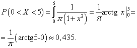
∞ a) Find the value of c from the normalization condition: ∫ f(x)dx=1. Therefore, -∞ https://pandia.ru/text/78/455/images/image032_23.gif" height="38 src="> -∞ 2 2 x if 2<х≤6, то F(x)= ∫ 0dx+∫ 1/8(х-2)dx=1/8(х2/2-2х) = 1/8(х2/2-2х - (4/2-4))= 1/8(x2/2-2x+2)=1/16(x-2)2; Gif" width="14" height="62"> 0 for x≤2, F (x) \u003d (x-2) 2/16 at 2<х≤6, 1 for x>6. The graph of the function F(x) is shown in Fig. 3 https://pandia.ru/text/78/455/images/image034_23.gif" width="14" height="62 src="> 0 for x≤0, F (x) \u003d (3 arctg x) / π at 0<х≤√3, 1 for x>√3. Find the differential distribution function f(x) Solution:
Since f (x) \u003d F '(x), then https://pandia.ru/text/78/455/images/image011_36.jpg" width="118" height="24"> All the properties of mathematical expectation and dispersion considered earlier for dispersed random variables are also valid for continuous ones. Task number 3. The random variable X is given by the differential function f(x): https://pandia.ru/text/78/455/images/image036_19.gif" height="38"> -∞ 2 X3/9 + x2/6 = 8/9-0+9/6-4/6=31/18, https://pandia.ru/text/78/455/images/image032_23.gif" height="38"> +∞ D(X)= ∫ x2 f(x)dx-(M(x))2=∫ x2 x/3 dx+∫1/3x2 dx=(31/18)2=x4/12 +x3/9 - - (31/18)2=16/12-0+27/9-8/9-(31/18)2=31/9- (31/18)2==31/9(1-31/36)=155/324, https://pandia.ru/text/78/455/images/image032_23.gif" height="38"> P(1<х<5)= ∫ f(x)dx=∫ х/3 dx+∫ 1/3 dx+∫ 0 dx= х2/6 +1/3х = 4/6-1/6+1-2/3=5/6. Tasks for independent solution.
2.1.
A continuous random variable X is given by a distribution function: 0 for x≤0, F(x)= https://pandia.ru/text/78/455/images/image038_17.gif" width="14" height="86"> 0 for x≤ π/6, F(х)= - cos 3x at π/6<х≤ π/3, 1 for x> π/3. Find the differential distribution function f(x) and also Р(2π /9<Х< π /2). 2.3.
0 for x≤2, f(x)= with x at 2<х≤4, 0 for x>4. 2.4.
A continuous random variable X is given by the distribution density: 0 for x≤0, f(х)= с √х at 0<х≤1, 0 for x>1. Find: a) the number c; b) M(X), D(X). 2.5.
https://pandia.ru/text/78/455/images/image041_3.jpg" width="36" height="39"> for x, 0 at x . Find: a) F(x) and plot its graph; b) M(X),D(X), σ(X); c) the probability that in four independent trials the value X will take exactly 2 times the value belonging to the interval (1; 4). 2.6.
The probability distribution density of a continuous random variable X is given: f (x) \u003d 2 (x-2) for x, 0 at x . Find: a) F(x) and plot its graph; b) M(X),D(X), σ(X); c) the probability that in three independent tests the value X will take exactly 2 times the value belonging to the interval . 2.7.
The function f(x) is given as: https://pandia.ru/text/78/455/images/image045_4.jpg" width="43" height="38 src=">.jpg" width="16" height="15">[-√ 3/2; √3/2]. 2.8.
The function f(x) is given as: https://pandia.ru/text/78/455/images/image046_5.jpg" width="45" height="36 src="> .jpg" width="16" height="15">[- π /four ; π /4]. Find: a) the value of the constant c, at which the function will be the probability density of some random variable X; b) distribution function F(x). 2.9.
Random variable Х, concentrated on the interval (3;7), is given by the distribution function F(х)= . Find the probability that random variable X will take the value: a) less than 5, b) not less than 7. 2.10.
Random variable X, concentrated on the interval (-1; 4), given by the distribution function F(x)= . Find the probability that random variable X will take the value: a) less than 2, b) not less than 4. 2.11.
https://pandia.ru/text/78/455/images/image049_6.jpg" width="43" height="44 src="> .jpg" width="16" height="15">. Find: a) the number c; b) M(X); c) probability P(X > M(X)). 2.12.
The random variable is given by the differential distribution function: https://pandia.ru/text/78/455/images/image050_3.jpg" width="60" height="38 src=">.jpg" width="16 height=15" height="15"> . Find: a) M(X); b) probability Р(Х≤М(Х)) 2.13.
The Time distribution is given by the probability density: https://pandia.ru/text/78/455/images/image052_5.jpg" width="46" height="37"> for x ≥0. Prove that f(x) is indeed a probability density distribution. 2.14.
The probability distribution density of a continuous random variable X is given: https://pandia.ru/text/78/455/images/image054_3.jpg" width="174" height="136 src="> (fig.4) 2.16.
The random variable X is distributed according to the “right-angled triangle” law in the interval (0; 4) (Fig. 5). Find an analytical expression for the probability density f(x) on the entire real axis. Answers
0 for x≤0, f(x)= https://pandia.ru/text/78/455/images/image038_17.gif" width="14" height="86"> 0 for x≤ π/6, F(x)= 3sin 3x at π/6<х≤ π/3, 0 for x> π/3. A continuous random variable X has a uniform distribution law on a certain interval (a;b), to which all possible values of X belong, if the probability distribution density f(x) is constant on this interval and is equal to 0 outside it, i.e. 0 for x≤a, f(x)= for a<х 0 for x≥b. The graph of the function f(x) is shown in fig. one F(х)= https://pandia.ru/text/78/455/images/image077_3.jpg" width="30" height="37">, D(X)=, σ(Х)=. Task number 1. The random variable X is uniformly distributed on the segment . Find: a) the probability distribution density f(x) and build its graph; b) the distribution function F(x) and build its graph; c) M(X),D(X), σ(X). Solution:
Using the formulas discussed above, with a=3, b=7, we find: https://pandia.ru/text/78/455/images/image081_2.jpg" width="22" height="39"> at 3≤х≤7, 0 for x>7 Let's build its graph (Fig. 3): https://pandia.ru/text/78/455/images/image038_17.gif" width="14" height="86 src="> 0 for x≤3, F(х)= https://pandia.ru/text/78/455/images/image084_3.jpg" width="203" height="119 src=">fig.4 D(X) = ==https://pandia.ru/text/78/455/images/image089_1.jpg" width="37" height="43">==https://pandia.ru/text/ 78/455/images/image092_10.gif" width="14" height="49 src="> 0 for x<0, f(х)= λе-λх at х≥0. The distribution function of a random variable X, distributed according to an exponential law, is given by the formula: https://pandia.ru/text/78/455/images/image094_4.jpg" width="191" height="126 src=">fig..jpg" width="22" height="30"> , D(X)=, σ(X)= Thus, the mathematical expectation and the standard deviation of the exponential distribution are equal to each other. The probability of X falling into the interval (a;b) is calculated by the formula: Р(a<Х Task number 2. The average uptime of the device is 100 hours. Assuming that the uptime of the device has an exponential distribution law, find: a) probability distribution density; b) distribution function; c) the probability that the time of failure-free operation of the device will exceed 120 hours. Solution:
By condition, the mathematical distribution M(X)=https://pandia.ru/text/78/455/images/image098_10.gif" height="43 src="> 0 for x<0, a) f(x)= 0.01e -0.01x for x≥0. b) F(x)= 0 for x<0, 1-e -0.01x at x≥0. c) We find the desired probability using the distribution function: P(X>120)=1-F(120)=1-(1-e-1.2)=e-1.2≈0.3. §
3.Normal distribution law Definition:
A continuous random variable X has normal distribution law (Gaussian law),
if its distribution density has the form: where m=M(X), σ2=D(X), σ>0. The normal distribution curve is called normal or gaussian curve
(fig.7) The distribution function of a random variable X, distributed according to the normal law, is expressed through the Laplace function Ф (х) according to the formula: where is the Laplace function. Comment:
The function Ф(х) is odd (Ф(-х)=-Ф(х)), besides, if x>5, we can consider Ф(х) ≈1/2. The graph of the distribution function F(x) is shown in fig. eight https://pandia.ru/text/78/455/images/image106_4.jpg" width="218" height="33"> The probability that the absolute value of the deviation is less than a positive number δ is calculated by the formula: In particular, for m=0 the equality is true: "Three Sigma Rule"
If the random variable X has a normal distribution law with the parameters m and σ, then it is practically certain that its value lies in the interval (a-3σ; a+3σ), because https://pandia.ru/text/78/455/images/image110_2.jpg" width="157" height="57 src=">a) b) Let's use the formula: https://pandia.ru/text/78/455/images/image112_2.jpg" width="369" height="38 src="> According to the table of values of the function Ф(х) we find Ф(1.5)=0.4332, Ф(1)=0.3413. So the desired probability is: P(28 Tasks for independent work
3.1.
The random variable X is uniformly distributed in the interval (-3;5). Find: b) distribution function F(x); c) numerical characteristics; d) probability P(4<х<6). 3.2.
The random variable X is uniformly distributed on the segment . Find: a) distribution density f(x); b) distribution function F(x); c) numerical characteristics; d) probability Р(3≤х≤6). 3.3.
An automatic traffic light is installed on the highway, in which the green light is on for 2 minutes for vehicles, yellow for 3 seconds and red for 30 seconds, etc. The car passes along the highway at a random time. Find the probability that the car passes the traffic light without stopping. 3.4.
Subway trains run regularly at intervals of 2 minutes. The passenger enters the platform at a random time. What is the probability that the passenger will have to wait more than 50 seconds for the train? Find the mathematical expectation of a random variable X - the train's waiting time. 3.5.
Find the variance and standard deviation of the exponential distribution given by the distribution function: F(x)= 0 at x<0, 1-e-8x for x≥0. 3.6.
A continuous random variable X is given by the probability distribution density: f(x)=0 at x<0, 0.7 e-0.7x at x≥0. a) Name the law of distribution of the considered random variable. b) Find the distribution function F(X) and the numerical characteristics of the random variable X. 3.7.
The random variable X is distributed according to the exponential law, given by the probability distribution density: f(x)=0 at x<0, 0.4 e-0.4 x at x≥0. Find the probability that, as a result of the test, X will take a value from the interval (2.5; 5). 3.8.
A continuous random variable X is distributed according to the exponential law given by the distribution function: F(x)= 0 at x<0, 1st-0.6x at x≥0 Find the probability that, as a result of the test, X will take a value from the interval . 3.9.
The mathematical expectation and standard deviation of a normally distributed random variable are 8 and 2, respectively. Find: a) distribution density f(x); b) the probability that, as a result of the test, X will take a value from the interval (10;14). 3.10.
Random variable X is normally distributed with mean 3.5 and variance 0.04. Find: a) distribution density f(x); b) the probability that, as a result of the test, X will take a value from the interval . 3.11.
The random variable X is normally distributed with M(X)=0 and D(X)=1. Which of the events: |X|≤0.6 or |X|≥0.6 has a higher probability? 3.12.
The random variable X is normally distributed with M(X)=0 and D(X)=1. From which interval (-0.5;-0.1) or (1;2) in one test will it take on a value with a greater probability? 3.13.
The current price per share can be modeled using a normal distribution with M(X)=10den. units and σ (X)=0.3 den. units Find: a) the probability that the current share price will be from 9.8 den. units up to 10.4 den. units; b) using the "rule of three sigma" to find the boundaries in which the current price of the stock will be located. 3.14.
The substance is weighed without systematic errors. Random weighing errors are subject to the normal law with the root-mean-square ratio σ=5r. Find the probability that in four independent experiments the error in three weighings will not occur in absolute value 3r. 3.15.
The random variable X is normally distributed with M(X)=12.6. The probability of a random variable falling into the interval (11.4;13.8) is 0.6826. Find the standard deviation σ. 3.16.
The random variable X is normally distributed with M(X)=12 and D(X)=36. Find the interval in which, with a probability of 0.9973, the random variable X will fall as a result of the test. 3.17.
A part manufactured by an automatic machine is considered defective if the deviation X of its controlled parameter from the nominal value exceeds 2 units of measurement in modulo . It is assumed that the random variable X is normally distributed with M(X)=0 and σ(X)=0.7. What percentage of defective parts does the machine give out? 3.18.
The detail parameter X is normally distributed with a mathematical expectation of 2 equal to the nominal value and a standard deviation of 0.014. Find the probability that the deviation of X from the face value modulo does not exceed 1% of the face value. Answers
https://pandia.ru/text/78/455/images/image116_9.gif" width="14" height="110 src="> b) 0 for x≤-3, F(x)=left"> 3.10.
a)f(x)= , b) Р(3.1≤Х≤3.7) ≈0.8185. 3.11.
|x|≥0.6. 3.12.
(-0,5;-0,1). 3.13.
a) Р(9.8≤Х≤10.4) ≈0.6562. 3.14.
0,111. 3.15.
σ=1.2. 3.16.
(-6;30). 3.17.
0,4%. Random variable A quantity is called that, as a result of tests carried out under the same conditions, takes on different, generally speaking, values, depending on random factors that are not taken into account. Examples of random variables: the number of points dropped on a dice, the number of defective items in a batch, the deviation of the point of impact of the projectile from the target, the uptime of the device, etc. Distinguish between discrete and continuous random variables. Discrete A random variable is called, the possible values of which form a countable set, finite or infinite (i.e., a set whose elements can be numbered). continuous A random variable is called, the possible values of which continuously fill some finite or infinite interval of the numerical axis. The number of values of a continuous random variable is always infinite. Random variables will be denoted by capital letters of the end of the Latin alphabet: X,
Y, ...; values of a random variable - in lowercase letters: X, y... . In this way, X
Denotes the entire set of possible values of a random variable, and X - Some specific meaning. distribution law A discrete random variable is a correspondence given in any form between the possible values of a random variable and their probabilities. Let the possible values of the random variable X
Are . As a result of the test, the random variable will take one of these values, i.e. One event from a complete group of pairwise incompatible events will occur. Let also the probabilities of these events be known: Distribution law of a random variable X
It can be written in the form of a table called Near distribution Discrete random variable: The distribution series is equal (normalization condition). Example 3.1. Find the distribution law of a discrete random variable X
- the number of occurrences of the "eagle" in two coin tosses. The distribution function is a universal form of setting the distribution law for both discrete and continuous random variables. The distribution function of a random variableX
The function is called F(X),
Defined on the whole number line as follows: F(X)= P(X< х
), i.e. F(X) there is a probability that the random variable X
Takes on a value less than X.
The distribution function can be represented graphically. For a discrete random variable, the graph has a stepped form. Let's build, for example, a graph of the distribution function of a random variable given by the following series (Fig. 3.1): Rice. 3.1. Graph of the distribution function of a discrete random variable Jumps of the function occur at points corresponding to the possible values of the random variable, and are equal to the probabilities of these values. At break points, the function F(X) is continuous on the left. The plot of the distribution function of a continuous random variable is a continuous curve. Rice. 3.2. Graph of the distribution function of a continuous random variable The distribution function has the following obvious properties: 1) 4) We will call an event consisting in the fact that a random variable X
Takes on a value X, Belonging to some semi-closed interval A£
X<
B,
By hitting a random variable on the interval [ A,
B).
Theorem 3.1. The probability of a random variable falling into the interval [ A,
B) is equal to the increment of the distribution function on this interval: If we decrease the interval [ A,
B),
Assuming that , then in the limit, formula (3.1) instead of the probability of hitting the interval gives the probability of hitting the point, i.e., the probability that the random variable takes on the value A: If the distribution function has a discontinuity at the point A,
Then the limit (3.2) is equal to the jump value of the function F(X) at the point X=A,
That is, the probabilities that the random variable will take on the value A
(Fig. 3.3, BUT).
If the random variable is continuous, i.e., the function is continuous F(X), then the limit (3.2) is equal to zero (Fig. 3.3, B) Thus, the probability of any particular value of a continuous random variable is zero. However, this does not mean that the event is impossible. X=A,
It only says that the relative frequency of this event will tend to zero with an unlimited increase in the number of tests. BUT) Rice. 3.3. Distribution function jump For continuous random variables, along with the distribution function, another form of specifying the distribution law is used - the distribution density. If is the probability of hitting the interval , then the ratio characterizes the density with which the probability is distributed in the vicinity of the point X. The limit of this relation at , i.e. e. derivative, is called Distribution density(density of probability distribution, probability density) of a random variable X. We agree to denote the distribution density Thus, the distribution density characterizes the probability that a random variable will fall into the vicinity of the point X. The plot of the distribution density is called crooked racesDefinitions(Figure 3.4). Rice. 3.4. Distribution density type Based on the definition and properties of the distribution function F(X), it is easy to establish the following properties of the distribution density F(X):
1) F(X)³0 2) 3) 4) For a continuous random variable, due to the fact that the probability of hitting a point is zero, the following equalities hold: Example 3.2. Random value X
Specified by the distribution density Required: A) find the value of the coefficient BUT; B) find the distribution function; C) find the probability of a random variable falling into the interval (0, ). The distribution function or distribution density completely describes a random variable. Often, however, when solving practical problems, there is no need for complete knowledge of the law of distribution, it is enough to know only some of its characteristic features. To do this, in the theory of probability, numerical characteristics of a random variable are used, expressing various properties of the distribution law. The main numerical characteristics are MathematicalExpectation, variance and standard deviation. Expected value Characterizes the position of a random variable on the number axis. This is some average value of a random variable around which all its possible values are grouped. Mathematical expectation of a random variable X
Symbolized M(X) or T. The mathematical expectation of a discrete random variable is the sum of paired products of all possible values of the random variable and the probabilities of these values: The mathematical expectation of a continuous random variable is determined using an improper integral: Based on the definitions, it is easy to verify the validity of the following properties of the mathematical expectation: 1. (mathematical expectation of a non-random variable FROM Equal to the most non-random value). 2. If ³0, then ³0. 4. If and independent, then . Example 3.3. Find the mathematical expectation of a discrete random variable given by a series of distributions: Solution. Example 3.4. Find the mathematical expectation of a random variable given by the distribution density: Solution. Dispersion and standard deviation They are characteristics of the dispersion of a random variable, they characterize the spread of its possible values relative to the mathematical expectation. dispersion D(X)
random variable X
The mathematical expectation of the squared deviation of a random variable from its mathematical expectation is called. For a discrete random variable, the variance is expressed by the sum: And for continuous - integral The variance has the dimension of the square of a random variable. scattering characteristic, Matching in sizeStee with random variable, is the standard deviation. Dispersion properties: 1) are constant. In particular, 3) In particular, Note that the calculation of the variance by formula (3.5) often turns out to be more convenient than by formula (3.3) or (3.4). The value is called covariance random variables. If a called Correlation coefficient random variables. It can be shown that if Note that if they are independent, then Example 3.5. Find the variance of a random variable given by the distribution series from Example 1. Solution. To calculate the variance, you need to know the mathematical expectation. For a given random variable above, it was found: M=1.3. We calculate the variance using the formula (3.5): Example 3.6. The random variable is given by the distribution density Find the variance and standard deviation. Solution. We first find the mathematical expectation: (as an integral of an odd function over a symmetric interval). Now we calculate the variance and standard deviation: 1. Binomial distribution. The random variable , equal to the number of "SUCCESSES" in the Bernoulli scheme, has a binomial distribution: The mathematical expectation of a random variable distributed according to the binomial law is The variance of this distribution is . 2. Poisson distribution Mathematical expectation and variance of a random variable with Poisson distribution , . The Poisson distribution is often used when we are dealing with the number of events that occur in a span of time or space, such as the number of cars arriving at a car wash in an hour, the number of machine stops per week, the number of traffic accidents, etc. The random variable has Geometric distribution with parameter if takes values with probabilities 3. Normal distribution.
The normal law of probability distribution occupies a special place among other distribution laws. In probability theory, it is proved that the probability density of the sum of independent or Weakly dependent, uniformly small (i.e., playing approximately the same role) terms with an unlimited increase in their number approaches the normal distribution law as close as desired, regardless of what distribution laws these terms have (the central limit theorem of A. M. Lyapunov). RANDOM VALUES Example 2.1. Random value X given by the distribution function Find the probability that as a result of the test X will take values between (2.5; 3.6). Solution: X in the interval (2.5; 3.6) can be determined in two ways: Example 2.2. At what values of the parameters BUT and AT function F(x) = A + Be - x can be a distribution function for non-negative values of a random variable X. Solution: Since all possible values of the random variable X belong to the interval , then in order for the function to be a distribution function for X, the property should hold: Answer: Example 2.3. The random variable X is given by the distribution function Find the probability that, as a result of four independent trials, the value X exactly 3 times will take a value belonging to the interval (0.25; 0.75). Solution: Probability of hitting a value X in the interval (0.25; 0.75) we find by the formula: Example 2.4. The probability of the ball hitting the basket in one throw is 0.3. Draw up the law of distribution of the number of hits in three throws. Solution: Random value X- the number of hits in the basket with three throws - can take on the values: 0, 1, 2, 3. The probabilities that X X: Example 2.5. Two shooters make one shot at the target. The probability of hitting it by the first shooter is 0.5, the second - 0.4. Write down the law of distribution of the number of hits on the target. Solution: Find the law of distribution of a discrete random variable X- the number of hits on the target. Let the event be a hit on the target by the first shooter, and - hit by the second shooter, and - respectively, their misses. Let us compose the law of probability distribution of SV X: Example 2.6. 3 elements are tested, working independently of each other. Durations of time (in hours) of failure-free operation of elements have distribution density functions: for the first: F 1 (t) =1-e- 0,1 t, for the second: F 2 (t) = 1-e- 0,2 t, for the third one: F 3 (t) =1-e- 0,3 t. Find the probability that in the time interval from 0 to 5 hours: only one element will fail; only two elements will fail; all three elements fail. Solution: Let's use the definition of the generating function of probabilities: The probability that in independent trials, in the first of which the probability of occurrence of an event BUT equals , in the second, etc., the event BUT appears exactly once, is equal to the coefficient at in the expansion of the generating function in powers of . Let's find the probabilities of failure and non-failure, respectively, of the first, second and third element in the time interval from 0 to 5 hours: Let's create a generating function: The coefficient at is equal to the probability that the event BUT will appear exactly three times, that is, the probability of failure of all three elements; the coefficient at is equal to the probability that exactly two elements will fail; coefficient at is equal to the probability that only one element will fail. Example 2.7. Given a probability density f(x) random variable X: Find the distribution function F(x). Solution: We use the formula: Thus, the distribution function has the form: Example 2.8. The device consists of three independently operating elements. The probability of failure of each element in one experiment is 0.1. Compile the law of distribution of the number of failed elements in one experiment. Solution: Random value X- the number of elements that failed in one experiment - can take the values: 0, 1, 2, 3. Probabilities that X takes these values, we find by the Bernoulli formula: Thus, we obtain the following law of the probability distribution of a random variable X: Example 2.9. There are 4 standard parts in a lot of 6 parts. 3 items were randomly selected. Draw up the law of distribution of the number of standard parts among the selected ones. Solution: Random value X- the number of standard parts among the selected ones - can take the values: 1, 2, 3 and has a hypergeometric distribution. The probabilities that X where --
the number of parts in the lot; --
the number of standard parts in the lot; –
number of selected parts; --
the number of standard parts among those selected. Example 2.10. The random variable has a distribution density where and are not known, but , a and . Find and . Solution: In this case, the random variable X has a triangular distribution (Simpson distribution) on the interval [ a, b]. Numerical characteristics X: Consequently, Answer: Example 2.11. On average, for 10% of contracts, the insurance company pays the sums insured in connection with the occurrence of an insured event. Calculate the mathematical expectation and variance of the number of such contracts among four randomly selected ones. Solution: The mathematical expectation and variance can be found using the formulas: Possible values of SV (number of contracts (out of four) with the occurrence of an insured event): 0, 1, 2, 3, 4. We use the Bernoulli formula to calculate the probabilities of a different number of contracts (out of four) for which the sums insured were paid: The distribution series of CV (the number of contracts with the occurrence of an insured event) has the form: Answer: , . Example 2.12. Of the five roses, two are white. Write a distribution law for a random variable expressing the number of white roses among two taken at the same time. Solution: In a sample of two roses, there may either be no white rose, or there may be one or two white roses. Therefore, the random variable X can take values: 0, 1, 2. The probabilities that X takes these values, we find by the formula: where --
number of roses; --
number of white roses; –
the number of simultaneously taken roses; --
the number of white roses among those taken. Then the law of distribution of a random variable will be as follows: Example 2.13. Among the 15 assembled units, 6 need additional lubrication. Draw up the law of distribution of the number of units in need of additional lubrication, among five randomly selected from the total number. Solution: Random value X- the number of units that need additional lubrication among the five selected - can take the values: 0, 1, 2, 3, 4, 5 and has a hypergeometric distribution. The probabilities that X takes these values, we find by the formula: where --
the number of assembled units; --
number of units requiring additional lubrication; –
the number of selected aggregates; --
the number of units that need additional lubrication among the selected ones. Then the law of distribution of a random variable will be as follows: Example 2.14. Of the 10 watches received for repair, 7 need a general cleaning of the mechanism. Watches are not sorted by type of repair. The master, wanting to find a watch that needs cleaning, examines them one by one and, having found such a watch, stops further viewing. Find the mathematical expectation and variance of the number of hours watched. Solution: Random value X- the number of units that need additional lubrication among the five selected - can take the following values: 1, 2, 3, 4. The probabilities that X takes these values, we find by the formula: Then the law of distribution of a random variable will be as follows: Now let's calculate the numerical characteristics of the quantity : Answer: , . Example 2.15. The subscriber has forgotten the last digit of the phone number he needs, but remembers that it is odd. Find the mathematical expectation and variance of the number of dials he made before hitting the desired number, if he dials the last digit at random and does not dial the dialed digit in the future. Solution: Random variable can take values: . Since the subscriber does not dial the dialed digit in the future, the probabilities of these values are equal. Let's compose a distribution series of a random variable: Let's calculate the mathematical expectation and variance of the number of dialing attempts: Answer: , . Example 2.16. The probability of failure during the reliability tests for each device of the series is equal to p. Determine the mathematical expectation of the number of devices that failed, if tested N appliances. Solution: Discrete random variable X is the number of failed devices in N independent tests, in each of which the probability of failure is equal to p, distributed according to the binomial law. The mathematical expectation of the binomial distribution is equal to the product of the number of trials and the probability of an event occurring in one trial: Example 2.17. Discrete random variable X takes 3 possible values: with probability ; with probability and with probability . Find and knowing that M( X) = 8. Solution: We use the definitions of mathematical expectation and the law of distribution of a discrete random variable: We find: . Example 2.18. The technical control department checks products for standardity. The probability that the item is standard is 0.9. Each batch contains 5 items. Find the mathematical expectation of a random variable X- the number of batches, each of which contains exactly 4 standard products, if 50 batches are subject to verification. Solution: In this case, all experiments conducted are independent, and the probabilities that each batch contains exactly 4 standard products are the same, therefore, the mathematical expectation can be determined by the formula: where is the number of parties; The probability that a batch contains exactly 4 standard items. We find the probability using the Bernoulli formula: Answer: Example 2.19. Find the variance of a random variable X– number of occurrences of the event A in two independent trials, if the probabilities of the occurrence of an event in these trials are the same and it is known that M(X) = 0,9. Solution: The problem can be solved in two ways. 1) Possible CB values X: 0, 1, 2. Using the Bernoulli formula, we determine the probabilities of these events: ,
Then the distribution law X looks like: From the definition of mathematical expectation, we determine the probability: Let's find the variance of SW X: 2) You can use the formula: Answer: Example 2.20. Mathematical expectation and standard deviation of a normally distributed random variable X are 20 and 5, respectively. Find the probability that as a result of the test X will take the value contained in the interval (15; 25). Solution: Probability of hitting a normal random variable X on the section from to is expressed in terms of the Laplace function: Example 2.21. Given a function: At what value of the parameter C this function is the distribution density of some continuous random variable X? Find the mathematical expectation and variance of a random variable X. Solution: In order for a function to be the distribution density of some random variable , it must be non-negative, and it must satisfy the property: Consequently: Calculate the mathematical expectation using the formula: Calculate the variance using the formula: T is p. It is necessary to find the mathematical expectation and variance of this random variable. Solution: The distribution law of a discrete random variable X - the number of occurrences of an event in independent trials, in each of which the probability of the occurrence of an event is , is called binomial. The mathematical expectation of the binomial distribution is equal to the product of the number of trials and the probability of the occurrence of the event A in one trial: Example 2.25. Three independent shots are fired at the target. The probability of hitting each shot is 0.25. Determine the standard deviation of the number of hits with three shots. Solution: Since three independent trials are performed, and the probability of occurrence of the event A (hit) in each trial is the same, we will assume that the discrete random variable X - the number of hits on the target - is distributed according to the binomial law. The variance of the binomial distribution is equal to the product of the number of trials and the probabilities of occurrence and non-occurrence of an event in one trial: Example 2.26. The average number of clients visiting the insurance company in 10 minutes is three. Find the probability that at least one customer arrives in the next 5 minutes. Average number of customers arriving in 5 minutes: Example 2.29. The waiting time for an application in the processor queue obeys an exponential distribution law with an average value of 20 seconds. Find the probability that the next (arbitrary) request will wait for the processor for more than 35 seconds. Solution: In this example, the expectation Then the desired probability is: Example 2.30. A group of 15 students holds a meeting in a hall with 20 rows of 10 seats each. Each student takes a seat in the hall at random. What is the probability that no more than three people will be in the seventh place in the row? Solution: Example 2.31. Then according to the classical definition of probability: where --
the number of parts in the lot; --
the number of non-standard parts in the lot; –
number of selected parts; --
the number of non-standard parts among the selected ones. Then the distribution law of the random variable will be as follows.

 1.2.
p4=0.1; 0 for x≤-1,
1.2.
p4=0.1; 0 for x≤-1,

 (fig.5)
 https://pandia.ru/text/78/455/images/image038_17.gif" width="14" height="86"> 0 for x≤a,
 ,
, The normal curve is symmetrical with respect to the straight line x=m, has a maximum at x=a equal to .
![]() ,
,![]()
![]()


 X
X![]() , 2) , 3) ,
, 2) , 3) ,![]() at .
at .
 B)
B) .
.


 =0×0.2 + 1×0.4 + 2×0.3 + 3×0.1=1.3.
 .
.![]() (3.3)
(3.3) (3.4)
(3.4)
![]() , then the value
, then the value
![]() , then the quantities are linearly dependent: where
, then the quantities are linearly dependent: where ![]()


![]() ,
, ![]() .
. .
. ,
, ![]() . A random variable with such a distribution makes sense Numbers of the first successful test in the Bernoulli scheme with the probability of success . The distribution table looks like:
. A random variable with such a distribution makes sense Numbers of the first successful test in the Bernoulli scheme with the probability of success . The distribution table looks like:
![]() .
.![]() .
.

![]() .
.

![]() .
.![]() .
.![]() .
.

![]() . Solving this system, we get two pairs of values: . Since, according to the condition of the problem, we finally have:
. Solving this system, we get two pairs of values: . Since, according to the condition of the problem, we finally have: ![]() .
.![]() .
.![]() .
.![]() .
.
0,6561
0,2916
0,0486
0,0036
0,0001
![]() .
.![]() .
.![]() .
.
![]() .
.![]() .
.![]() .
.![]() .
.![]() .
.![]() .
.
![]() .
.![]() .
.![]() .
.![]() .
.
0,2

![]() ,
,![]() .
.![]() ,
.
,
.
![]() .
.![]() .
.![]() .
.
![]() .
.
![]() .
.![]() .
.![]()
![]()
![]() . .
. .
![]() , and the failure rate is .
, and the failure rate is .